Chapter 7 Comparison of Two or More Groups by Analysis of Variance
7.1 Complete randomization
A planter wanted to compare the effects of five site-preparation treatments on the early height growth of planted pine seedlings. He laid out 25 plots, and applied each treatment to 5 randomly selected plots. The plots were then hand-planted and at the end of 5 years the height of all pines was measured and an average height computed for each plot. The plot averages (in feet) were as follows:
| Plots | Treatment A | Treatment B | Treatment C | Treatment D | Treatment E | |
|---|---|---|---|---|---|---|
| Plot 1 | 15 | 16 | 13 | 11 | 14 | |
| Plot 2 | 14 | 14 | 12 | 13 | 12 | |
| Plot 3 | 12 | 13 | 11 | 10 | 12 | |
| Plot 4 | 13 | 15 | 12 | 12 | 10 | |
| Plot 5 | 13 | 14 | 10 | 11 | 11 | |
| Sums | 67 | 72 | 58 | 57 | 59 | 313 |
| Treatment Means | 13.4 | 14.4 | 11.6 | 11.4 | 11.8 | 12.52 |
Looking at the data we see that there are differences among the treatment means: \(A\) and \(B\) have higher averages than \(C\), \(D\), and \(E\). Soils and planting stock are seldom completely uniform, however, and so we would expect some differences even if every plot had been given exactly the same site-preparation treatment. The question is, can differences as large as this occur strictly by chance if there is actually no difference among treatments? If we decide that the observed differences are larger than might be expected to occur strictly by chance, the inference is that the treatments are not equal. Statistically speaking, we reject the hypothesis of no difference among treatment means.
Problems like this are neatly handled by an analysis of variance. To make this analysis, we need to fill in a table like the following:
| Source of variation | Degrees of Freedom | Sum of Squares | Mean Squares |
|---|---|---|---|
| Treatments | 4 | ||
| Error | 20 | ||
| Total | 24 |
Source of variation–There are a number of reasons why the height growth of these 25 plots might vary, but only one can be definitely identified and evaluated–that attribute to treatments. The unidentified variation is assumed to represent the variation inherent in the experimental material and is labeled error. Thus, total variation is being divided into two parts: one part attribute to treatments, and the other unidentified and called error.
Degrees of freedom–Degrees of freedom are hard to explain in nonstatistical language. In the simpler analyses of variance, however, they are not difficult to determine. For the total, the degrees of freedom are one less than the number of observations: there are 25 plots, so the total has 24 dfs. For the sources, other than error, the dfs are one less than the number of classes or groups recognized in the source. Thus, in the source labeled treatments there are five groups (five treatments), so there will be four degrees of freedom for treatments. The remaining degrees of freedom \((24-4=20)\) are associated with error term.
Sums of squares–There is a sum of squares associated with every source of variation. These SS are easily calculated in the following steps:
First we need what is known as a “correction term” or C.T. This is simply: \[C.T.=\frac {(\Sigma^n X)^2}{n}=\frac {313^2}{25}=3918.76\]
where:
*\(\Sigma^n\)=the sum of \(n\) items
Then the total sum of squares is: \[\text {Total SS}_{24 df}=\Sigma X^2-C.T.=(15^2+14^2+...+11^2)-C.T.=64.24\]
The sum of squares attributable to treatments is:
\[\text {Treatment SS}_{4df}=\frac {\Sigma^5 (\text {treatment totals}^2)}{\text {No. of plots per treatment}}-C.T.\]
\[=\frac {67^2+72^2+...+59^2}{5}-C.T.=\frac {19767}{5}-C.T.=34.64\]
Note than in both SS calculations, the number of items squared and added was one more than the number of degrees of freedom associated with the sum of squares. The number of degrees of freedom just below the SS and the numbers of items to be squared and added just over the \(\Sigma\), provided a partial check as to whether the proper totals are being used in the calculation–the degrees of freedom must be on less than the number of items.
Not also that the divisor in the treatment SS calculation is equal to the number of individual items that go to make up each of the totals being squared in the numerator. This was also true in the calculation of total SS, but there the divisor was 1 and hence did not have to be shown. Note further that the divisor times the number over the summation sign (5x5=25 for treatments) must always be equal to the total number of observations in the test–another check.
The sum of squares for error is obtained by subtracting the treatment SS from total SS. A good habit to get into when obtaining sums of squares by subtraction is to perform the same subtraction using dfs. In the more complex designs, doinig this provides a partial check on whether the right items are being used.
Mean squares–The mean squares are now calculated by dividing the sums of squares by the associated degrees of freedom. It is not necessary to calculate the mean square for the total.
The items that have been calculated are entered directly into the analysis table, which at the present stage would look like this:
| Source of variation | Degrees of Freedom | Sum of Squares | Mean Squares |
|---|---|---|---|
| Treatments | 4 | 34.64 | 8.66 |
| Error | 20 | 29.60 | 1.48 |
| Total | 24 | 64.24 |
An \(F\) test of treatments is now made by dividing the MS for treatments by the MS for error in this case: \[F=\frac {8.66}{1.48}=5.851\]
This figure is compared to the appropriate value of \(F\) in table 3 of the appendix. Look across the top to the column headed 4 (corresponding to the degrees of freedom for treatments). Follow down the column to the row labeled 20 (corresponding to the degrees of freedom for error). The tabular \(F\) for significance at the 0.05 level is 2.87, and that for the 0.01 level is 4.43. As the calculated value of \(F\) exceeds 4.43, we conclude that the difference in height growth between treatments is significant at the 0.01 level. (More precisely, we reject the hypothesis that there is no difference in mean height growth between the treatments.) If \(F\) had been smaller than 4.43 but larger than 2.87, we would have said that the difference is significant at the 0.05 level. If \(F\) had been less than 2.87, we would have said that the difference between treatments is not significant at the 0.05 level. The researcher should select his own level of significance (preferably in advance of the study), keeping in mind that significance at the \(\alpha\) (alpha) level (for example) means this: if there is actually no difference among treatments, the probability of getting chance differences as large as those observed is \(\alpha\) or less.
The t test versus the analysis of variance–If only two treatments are being compared, the analysis of variance of a completely randomized design and the \(t\) test of unpaired plots lead to othe same conclusion. The choice of test is strictly one of personal preference, as may be verified by applying the analysis of variance to the data used to illustrate the \(t\) test of unpaired plots. The resulting \(F\) value will be equal to the square of the value of \(t\) that was obtained (i.e., \(F=t^2\)).
Like the \(t\) test, the \(F\) test is valid only if the variable observed is normally distributed and if all groups have the same variance.
7.2 Multiple Comparisons
In the example illustrating the completely randomized design, the difference among treatments was found to be significant at the 0.01 probability level. This is interesting as far as it goes, but usually we will want to take a closer look at the data, making comparisons among various combinations of the treatments.
Suppose, for example, that \(A\) and \(B\) involved some mechanical form of site preparation while \(C\), \(D\), and \(E\) were chemical treatments. Then we might want to test whether the average of \(A\) and \(B\) together differed from the combined average of \(C\), \(D\), and \(E\). Or, we might wish to test whether \(A\) and \(B\) differ significantly from each other. When the number of replications \((n)\) is the same for all treatments, such comparisons are fairly easy to define and test.
The question of whether the average of treatments \(A\) and \(B\) differs significantly from the average of treatments \(C\), \(D\), and \(E\) is equivalent to testing whether the linear contrast \[\hat Q=(3 \bar A+3 \bar B)-(2 \bar C+2 \bar D+2 \bar E)\]
differs significantly from zero (\(\bar A\)=the mean for treatment \(A\), etc.). Note that the coefficients of this contrast sum to zero \((3+3-2-2-2=0)\) and are selected so as to put the two means in the first group on an equal basis with the three means in the second group.
Similarly, testing whether treatment \(A\) differs significantly from treatment \(B\) is the same as testing whether the contrast \(\hat Q=\bar A-\bar B\) differs significantly from zero.
7.2.1 F test with single degree of freedom
A comparison specified in advance of the study (on logical grounds and before examination of the data) can be tested by an \(F\) test with single degree of freedom. For the linear contrast \[\hat Q=a_1 \bar X_1+a_2 \bar X_2+a_3 \bar X_3+...\]
among means based on the same number \((n)\) of observations, the sum of squares has one degree of freedom and is computed as \[SS_{1df}=\frac {n \hat Q^2}{\Sigma a_i^2}\]
This sum of squares divided by the mean square for error provides an \(F\) test of the comparison.
Thus, in testing \(A\) and \(B\) versus \(C\), \(D\), and \(E\) we have \[\hat Q=3(13.4)+3(14.4)-2(11.6)-2(11.4)-2(11.8)=13.8\]
and \[SS_{1df}=\frac {5(13.8)^2}{3^2+3^2+(-2)^2+(-2)^2+(-2)^2}=\frac {952.20}{30}=31.74\]
Then dividing by the error mean square gives the \(F\) value for testing the contrast. \[F=\frac {31.74}{1.48}=21.446 \text { with 1 and 20 degrees of freedom}\]
This exceeds the tabular value of \(F(4.35)\) at the 0.05 probability level. If this is the level at which we decided to test, we would reject the hypothesis that the mean of treatments \(A\) and \(B\) does not differ from the mean treatments \(C\), \(D\), and \(E\).
If \(\hat Q\) is expressed in terms of the treatment total rather than their means so that \[\hat Q_T=a_1(\Sigma X_1)+a_2(\Sigma X_2)+...\]
then the equation for the single degree of freedom sum of squares is: \[SS_{1 df}=\frac{\hat Q_T^2}{n \Sigma a^2_i}\]
The results will be the same as those obtained with the means. For the test of \(A\) and \(B\) versus \(C\), \(D\), and \(E\), \[\hat Q_t=3(67)+3(72)-2(58)-2(57)-2(59)=69\]
And, \[SS_{1 df}=\frac{69^2}{5[3^2+3^2(-2)^2+(-2)^2+(-2)^2]}=\frac{4761}{150}=31.74, \text { as before}.\]
Working with the totals saves the labor of computing means and avoids possible rounding errors.
7.2.2 Scheffé’s Test
Quite often we will want to test comparisons that were not anticipated before the data were collected. If the test of treatments was significant, such unplanned comparisons can be tested by the method of Scheffé. When there are \(n\) replications of each treatment, and \(v\) degrees of freedom for error, any linear contrast among the treatment means: \[\hat Q=a_1\bar X+a_2\bar X_2+...\]
is testing by computing \[F=\frac {n\hat Q^2}{k(\Sigma a^2_i)(\text {Error mean square})}\]
This value is then compared to the tabular value of \(F\) with \(k\) and \(v\) degrees of freedom.
For example, to test treatment \(B\) against the means of treatments \(C\) and \(E\) we would have \[\hat Q=[2\bar B-(\bar C+\bar E)]=[2(14.4)-11.6-11.8]=5.4\]
and \[F=\frac {5(5.4)^2}{(4)[2^2+(-1)^2+(-1)^2](1.48)}=4.05, \text { with 4 and 20 degrees of freedom}\]
This figure is larger than the tabular value of \(F(=2.87)\), and so in testing at the 0.05 level we would reject the hypothesis that the mean for treatment \(B\) did not differ from the combined average of treatments \(C\) and \(E\).
For a contrast \((Q_T)\) expressed in terms of treatment totals, the equation for \(F\) becomes \[F=\frac {\hat Q^2_T}{nk(\Sigma a^2_i)(\text {Error mean square})}\]
7.2.3 Unequal Replication
If the number of replications is not the same for all treatments, then for the linear contrast \[\hat Q=a_1\bar X_1+a_2\bar X_2+...\]
the sum of squares in the single degree of freedom \(F\) test is given by \[SS_{1df}={{\hat Q^2} \over (k)(\frac {a_1^2}{n_1}+\frac {a_2^2}{n_2}+...) \text {( Error mean square)}}\]
Selecting the coefficients \((a_i)\) for such contrasts can be tricky. When testing the hypothesis that there is no difference between the means of two groups of treatments, the positive coefficients are usually \[\text {positive } a_i=\frac {n_j}{m}\]
where \(p = \text {the total number of plots in the group of treatments with positive coefficients}.\)
The negative coefficients are \[\text {negative }a_i=\frac {n_j}{m}\]
where \(m = \text {the total number of plots in the group of treatments with negative coefficients}.\)
To illustrate, if we wish to compare the mean of treatments \(A\), \(B\), and \(C\) with the mean of treatments \(D\) and \(E\) and there are two plots of treatment \(A\), three of \(B\), five of \(C\), three of \(D\), and two of \(E\), then \(p=2+3+5=10, m=3+2=5\) and the contrast would be \[\hat Q = (\frac {2}{10}\bar A+\frac {3}{10}\bar B+\frac {5}{10}\bar C)-(\frac {3}{5}\bar D\frac {2}{5}\bar E)\]
7.3 Randomized Block Design
In the completely randomized design the error mean square is a measure of the variation among plots treated alike. It is in fact an average of the within-treatment variances, as may easily be verified by computation. If there is considerable variation among plots treated alike, the error mean square will be large and the \(F\) test for a given set of treatments is less likely to be significant. Only large differences among treatments will be detected as real and the experiment is said to be insensitive.
Often the error can be reduced (thus giving a more sensitive test) by use of a randomized block design in place of complete randomization. In this design, similar plots or plots that are close together, are grouped into blocks. Usually the number of plots in each block is the same as the number of treatments to be compared, though there are variations having two or more plots per treatment in each block. The blocks are recognized as a source of variation that is isolated in the analysis.
As an example, a randomized block design with five blocks was used to test the height growth of cottonwood cuttings from four selected parent trees. The field layout looked like this:

Each plot consisted of a planting of 100 cuttings of the clone assigned to that plot. When the trees were 5 years old the heights of all survivors were measured and an average computed for each plot.
The plot averages (in feet) by clones and blocks are summarized below:
| Block | Clone A | Clone B | Clone C | Clone D | Block Totals |
|---|---|---|---|---|---|
| I | 18 | 14 | 12 | 16 | 60 |
| II | 15 | 15 | 16 | 13 | 59 |
| III | 16 | 15 | 8 | 15 | 54 |
| IV | 14 | 12 | 10 | 12 | 48 |
| V | 12 | 14 | 9 | 14 | 49 |
| Clone Totals | 75 | 70 | 55 | 70 | 270 |
| Clone Means | 15 | 14 | 11 | 14 |
The hypothesis to be tested is that clones do not differ in mean height.
In this design there are two identifiable sources of variation–that are attributable to clones and that associated with blocks. The remaining portion of the total variation is used as a measure of experimental error.
The outline of the analysis is therefore as follows:
| Source of variation | df | Sum of Squares | Mean Squares |
|---|---|---|---|
| Blocks | 4 | ||
| Clones | 3 | ||
| Error | 12 | ||
| Total | 19 |
The breakdown in degrees of freedom and computation of the various sums of squares follow the same pattern as in the completely randomized design. Total degrees of freedom (19) are one less than the total number of plots. Degrees of freedom for clones (3) are one less than the number of clones. With five blocks, there will be 4 degrees of freedom for blocks. The remaining 12 degrees of freedom are associated with the error term.
Sums-of-squares calculations proceed as follows:
- The correction term \[C.T.=\frac {(\sum^{20} X)^2}{n}=\frac {270^2}{20}=3,645\]
- Total \(SS_{19df}=\sum^{20}X^2 - C.T.=(18^2+15^2+...+14^2)-C.T.= 3,766-3,645=121\)
- Clone \(SS_{3df}=\frac {\sum^4(\text {Clone totals}^2)}{\text {No. of plots per clone}}-C.T.\)
- Block \(SS_{4df}=\frac {\sum^4 (\text {Clone totals})^2}{\text {No. of plots per clone}}-C.T.=\frac {75^2+70^2+55^2+70^2}{5}-C.T.=3,690-3,645=45\)
- Error \(SS_{12df}=\text {Total }SS_{19df}-\text {Clone }SS_{3df}-\text {Block }SS_{4df}=45.5\)
Note that in obtaining the error SS by subtraction, we get a partial check on ourselves by subtracting clone and block df’s from the total df to see if we come out with the correct number for error df. If these don’t check, we have probably used the wrong sums of squares in the subtraction.
Mean squares are again calculated by dividing the sums of squares by the associated number of degrees of freedom.
Tabulating the results of these computations:
| Source | df | SS | MS |
|---|---|---|---|
| Blocks | 4 | 30.5 | 7.625 |
| Clones | 3 | 45.0 | 15.000 |
| Error | 12 | 45.5 | 3.792 |
| Total | 19 | 121.0 |
\(F\) for clones is obtained by dividing clone MS by error MS. In this case \(F=\frac {15.000}{3.792}=3.956\). As this is larger than the tabular \(F\) of 3.49 (\(F_{0.05}\)) with clones is significant at the 0.05 level. The significance appears to be due largely to the low value of \(C\) as compared to \(A\), \(B\), and \(D\).
Comparisons among clone means can be made by the methods previously described. For example, to test the prespecified (i.e., before examining the data) hypothesis that there is no difference between the mean of clone \(C\) and the combined average \(A\), \(B\), and \(D\) we would have: \[SS_{1df}\text { for } (A+B+D\text { vs. }C=\frac {5(3\bar C-\bar A-\bar B-\bar D)^2}{[3^2+(-1)^2+(-1)^2+(-1)^2]}=\frac {5(-10)^2}{12}=41.667\]
Then, \[F=\frac {41.667}{3.792}=10.988\]
Tabular \(F\) at the 0.01 level with 1 and 12 degrees of freedom is 9.33. As calculated \(F\) is greater than this, we conclude that the difference between \(C\) and the average of \(A\), \(B\), and \(D\) is significant at the 0.01 level.
The sum of squares for this single-degree-of-freedom comparison (41.667) is almost as large as that for clones (45.0) with three degrees of freedom. This result suggests that most of the clonal variation is attributable to the low value of \(C\), and that comparisons between the other three means are not likely to be significant.
There is usually no reason for testing blocks, but the size of the block mean square relative to the mean square for error does give an indication of how much precision was gained by blocking. If the block mean square is large (at least two or three times as large as the error mean square) the test is more sensitive than it would have been with complete randomization. If the block mean square is about equal to or only slightly larger than the error mean square, the use of blocks has not improved the precision of the test. The block mean square should not be appreciably smaller than the error mean square. If it is, the method of conducting the study and the computations should be re-examined.
Assumptions.–In addition to the assumptions of homogenous variance and normality, the randomized block design assumes that there is no interaction between treatments and blocks; i.e., that differences among treatments are about the same in all blocks. Because of this assumption, it is not advisable to have blocks that differ greatly–since they may cause an interaction with treatments.
N.B.: With only two treatments, the analysis of variance of a randomized block design is equivalent to the \(t\) test of paired replicates. The value of \(F\) will be equal to the value of \(t^2\) and the interference derived from the tests will be the same. The choice of tests is a matter of personal preference.
7.4 Latin Square Design
In the randomized block design the purpose of blocking is to isolate a recognizable extraneous source of variation. If successful, blocking reduces the error mean square and hence gives a more sensitive test than could be obtained by complete randomization.
In some situations, however, we have a two-way source of variation that cannot be isolated by blocks alone. In a field, for example, fertility gradients may exist both parallel to and at right angles to plowed rows. Simple blocking isolates only one of these sources of variation, leaving the other to swell the error term and reduce the sensitivity of the test.
When such a two-way source of extraneous variation is recognized or suspected, the Latin square design may be helpful. In this design, the total number of plots or experimental units is made equal to the square of the numbers of the treatments. In forestry and agriculture experiments, the plots are often (but not always) arranged in rows and columns with each row and column having a number of plots equal to the number of treatments being tested. The rows represent different levels of the other source of extraneous variation. Thus, before the assignment of treatments, the field layout of a Latin square for testing five treatments might look like a 5x5 square grid with 5 columns and 5 rows.
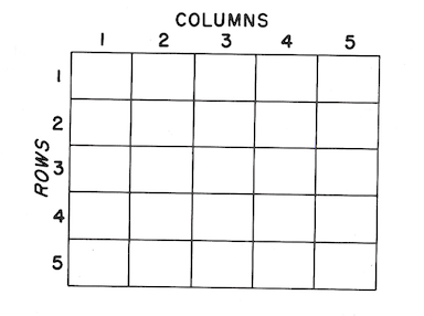
Treatments are assigned to plots at random, but with the very important restriction that a given treatment cannot appear more than once in any row or any column.
An example of a field layout of a Latin square for testing is given below. The letters represent the assignment of five treatments (which here are five species of hardwoods). The numbers show the average 5-year height growth by plots. The tabulation shows the total for rows, columns, and treatments.
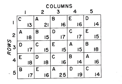
Below are the row column and treatment totals
| Row | \(\Sigma\) | Column | \(\Sigma\) | Treatment | \(\Sigma\) | \(\bar X\) |
|---|---|---|---|---|---|---|
| 1 | 80 | 1 | 83 | A | 95 | 19 |
| 2 | 82 | 2 | 85 | B | 80 | 16 |
| 3 | 80 | 3 | 89 | C | 75 | 15 |
| 4 | 82 | 4 | 81 | D | 85 | 17 |
| 5 | 91 | 5 | 77 | E | 80 | 16 |
| \(\Sigma=\) | 415 | \(\Sigma=\) | 415 | \(\Sigma=\) | 415 | 16.6 |
The partitioning of dfs, the calculation of sums of squares, and the subsequent analysis follow much the same pattern illustrated previously for randomized blocks.
\[C.T.=\frac {(\sum^{25} X)^2}{n}=\frac {415^2}{25}=\frac {172,225}{25}=6,889.0\]
\[\text {Total }SS_{24df}=\sum^{25} X^2-C.T.=7,041-C.T.=152.0\]
\[\text {Row }SS_{4df}=\frac {\sum^5(\text {Row totals}^2)}{\text {No. of plots per row}}-C.T.=\frac {34,529}{5}-C.T.=16.8\]
\[\text {Col. }SS_{4df}=\frac {\sum^5(\text {Column totals}^2)}{\text {No. of plots per column}}-C.T.=\frac {34,525}{5}-C.T.=16.0\]
\[\text {Species }SS_{4df}=\frac {\sum^5(\text {Species totals}^2)}{\text {No. of plots per species}}-C.T.=\frac {34,675}{5}-C.T.=46.0\]
\[\text {Error }SS_{12df}=\text {Total }SS_{24df}-\text {Species }SS_{4df}-\text {Row }SS_{4df}-\text {Col. }SS_{4df}\]
Below is the analysis of variance for rows, columns, species, and error
| Source | df | SS | MS |
|---|---|---|---|
| Rows | 4 | 16.8 | 4.2 |
| Columns | 4 | 16.0 | 4.0 |
| Species | 4 | 46.0 | 11.5 |
| Error | 12 | 73.2 | 6.1 |
| Total | 24 | 152.0 | |
| F (for species) | = \(\frac {11.5}{6.1}=1.885\) |
As the computed value of \(F\) is less than the tabular value of \(F\) at the 0.05 level (with 4/12 dfs), the difference among species are considered nonsignificant.
The Latin square design can be used whenever there is a two-way heterogeneity that cannot be controlled simply by blocking. In greenhouse studies, distance from a window could be treated as a row effect while distance from the blower or heater might be regarded as a column effect. Though the plots are often physically arranged in rows or columns this is not required. In testing the use of materials in a manufacturing process where different machines and machine operators will be involved, the variation between machines could be treated as a row effect and the variation due to operator as a column effect.
The Latin square should not be used if an interaction between rows and treatments or columns and treatments is suspected.
7.5 Factorial Experiments
In a comparison of corn yields following three rates or levels of nitrogen fertilization it was found that the yields depended on how much phosphorous was used along with the nitrogen. The differences in yield were smaller when no phosphorus was used along with nitrogen. The differences in yield were smaller when no phosphorous was used than when the nitrogen applications were accompanied by 100 pounds per acre of phosphorous. In statistics this situation is referred to as an interaction between nitrogen and phosphorous. Another example: when leaf litter was removed from the forest floor, the catch of pine seedlings was much greater than when the litter was not removed; but for red oak the reverse was true–the seedling catch was lower where litter was removed. Thus, species and litter treatment were interacting.
Interactions are important in the interpretation of study results. In the presence of an interaction between species and litter treatment is obviously makes no sense to talk about the effects of litter removal without specifying the species. The nitrogen-phosphorous interaction means that it may be misleading to recommend a level of nitrogen without mentioning the associated level of phosphorous.
Factorial experiments are aimed at evaluating known or suspected interactions. In these experiments, each factor is tested at all possible combinations of the levels of the other factors. In a planting test involving three species of trees and four methods of preplanting site preparation, each methods will be applied to each species, and the total number of treatment combinations will be 12. In a factorial test of the effects of two nursery treatments on the survival of four species of pine planted by three different methods, there would be 24 \((2x4x3=24)\) treatment combinations.
The method of analysis can be illustrated by a factorial test of the effects of three levels of nitrogen fertilization (0, 100, and 200 pounds per acre) on the growth of three species (\(A\), \(B\), and \(C\)) of planted pine. The nine possible treatment combinations were assigned at random to nine plots in each of three blocks. Treatments were evaluated on the basis of average annual height growth in inches per year over a 3-year period.
Field layout and plot data were as follows (with subscripts denoting nitrogen levels: 0=0, 1=100, 2=200):
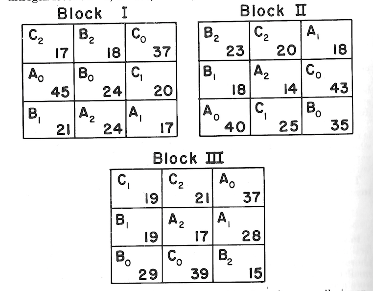
The preliminary analysis of the nine combinations (temporarily ignoring their factorial nature) is made just as though this were a straight randomized block design (which is exactly what is is). (See table, p. 41.)
Sum of squares \[C.T.=\frac {(\sum^{27} X)^2}{27}=\frac {683^2}{27}=17,277.3704\] Total \(SS_{26df}=\sum^{27} X^2-C.T.=(45^2+17^2+...+21^2)-C.T.=2,275.6296\) Block \(SS_{2df}={\frac {\sum^3(\text{Block totals}^2)}{\text{No. of plots per block}}-C.T.}=\frac {(223^2+236^2+224^2)}{9}-C.T.=11.6296\)
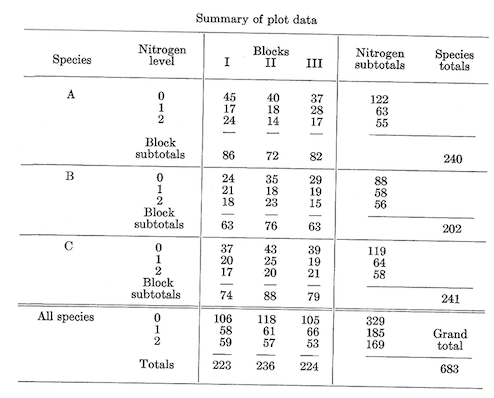
Treatment of \(SS_{8df}=\frac {\sum^9 (\text{No. of plots per treatment}^2)}{\text {No. of plots per treatment}}-C.T.=\frac {(122^2+63^2+...+58^2)}{3}-C.T.=1,970.2963\)
Error \(SS_{16df}=\text {Total SS}_{26df}-\text {Treatment SS}_{8df}-{\text {Block SS}_{2df}=293.7037}\)
Tabulating these in the usual form:
| Source | df | SS | MS |
|---|---|---|---|
| Blocks | 2 | 11.6296 | 5.8148 |
| Treatments | 8 | 1,970.2963 | 246.2870 |
| Error | 16 | 293.7037 | 18.3565 |
| Totals | 26 | 2,275.6296 |
Testing treatments: \(F_{8/16 df}=\frac {246.2870}{18.3565}=13.417\), significant at the 0.01 level.
The next step is to analyze the components of the treatment variability. How do the species compare? What is the effect of the treatment variability. How do the species compare? What is the effect of fertilization? And does fertilization affect all species the same way (i.e., is there a species-nitrogen interaction)? To answer these questions we have to partition the degrees of freedom and sums of squares associated with treatments. This is easily done by summarizing the data for the nine combinations in a two-way table.
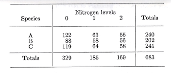
The nine individual values will be recognized as those that entered into the calculation of the treatment SS. Keeping in mind that each entry in the body of the table is the sum of three plot values, and that the species and nitrogen totals are ach the sum of 9 plots, the sums of squares for species, nitrogen, and the species-nitrogen interaction can be computed as follows:
Treatment \(SS_{8df}=1,970.2963\) (as previously calculated)
Species \(SS_{2df}=\frac {\sum^3(\text {species totals})^2}{\text {No. of plots per species}}-C.T.=\frac {(240^2+202^2+241^2)}{9}-C.T.=\frac {156,485}{9}-C.T.=109.8518\)
Nitrogen \(SS_{2df}=\frac {\sum^3(\text {Nitrogen totals})^2}{\text {No. of plots per level of nitrogen}}-C.T.=\frac {(329^2+185^2+169^2)}{9}-C.T.=\frac {171,027}{9}-C.T.=1,725.6296\)
Species-nitrogen interaction \(SS_{4df}=\text {Treatment SS}_{8df}-\text {Species SS}_{2df}-\text {Nitrogen SS}_{2df}=134.8149\)
The analysis now becomes:
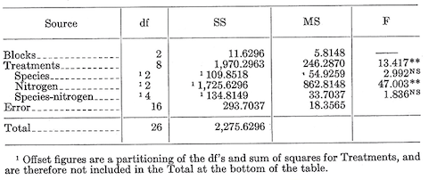
The degree of freedom for simple interactions can be obtained in two ways. The first way is by subtracting the dfs associated with the component factors (in this case two for species and two for nitrogen levels) from the dfs associated with all possible treatment combinations (eight in this case). The second way is to calculate the interaction dfs as the product of the component factor dfs (in this case 2x2=4). Do it both ways as a check.
The \(F\) values for species, nitrogen, and the species-nitrogen interaction are calculated by dividing their mean squares by the mean square for error. In the above tabulation, last column, NS indicated nonsignificant and ** means significant at the 0.01 level.
The analysis indicates a significant difference among levels of nitrogen, but no difference between species and no species-nitrogen interaction.
As before, a prespecified comparison among treatment means can be tested by breaking out the sum of squares associated with that comparison. To illustrate the computations, we will test nitrogen versus no nitrogen and also 100 pounds versus 200 pounds of nitrogen.
Nitrogen vs. no nitrogen \(SS_{1df}= {9[2(\frac {329}{9})-1(\frac {185}{9})-1(\frac {169}{9})]^2 \over (2^2+1^2+1^2)}=\frac {[2(329)-185-169]^2}{9(6)}=1,711.4074\)
In the numerator the mean for zero level of nitrogen is multiplied by 2 to give it equal weight with the mean of levels 1 and 2 with which it is compared. The 9 is the number of plots on which each mean is based. The (22+12+1^2) in the denominator is the sum of squares of the coefficients used in the numerator.
100 vs. 200 pounds \(SS_{1df}={9[1(\frac {185}{9})-1(\frac {169}{9})]^2 \over (1^2+1^2)}=\frac {[185-169]^2}{9(2)}=14.2222\)
Note that these two sums of squares (1,711.4074 and 14.2222), each with 1 df, add up to the sum of squares for nitrogen (1,725.6296) with 2 dfs. This additive characteristic hold true only if the individual df comparisons selected are orthogonal (i.e., independent). When the number of observations can be checked in the following manner: First, tabulate the coefficients and check to see that for each comparison the coefficients sum to zero.
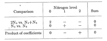
Then for two comparisons to be orthogonal the sum of the products of corresponding coefficients must be zero. Any sum of squares can be partitioned in a similar manner, with the number of possible orthogonal individual with df comparisons being equal to the total number of degrees of freedom with which the sum of squares be associated.
The sum of squares for species can also be partitioned into two orthogonal single df comparisons. If the comparisons were specified before the data were examined, we might make single df tests of the difference between B and the average of A and C and also of the difference between A and C. The method is the same as that illustrated in the comparison of nitrogen treatments. The calculations are as follows: \[\text {2B vs. (A+C) SS}_{1df}={9[1(\frac {240}{9})+1(\frac {241}{9})-2(\frac {202}{9})]^2 \over (1^2+1^2+2^2)}=\frac {[240+241-2(202)]^2}{9(6)}=109.7963\]
\[\text {A vs. C SS}_{1df}={9[1(\frac {241}{9})-1(\frac {240}{9})]^2 \over (1^2+1^2)}=\frac {[241-240]^2}{9(2)}=0.0555\]
These comparisons are orthogonal, so that the sums of squares each with one df add up to the species SS with two dfs.
Note than in computing the sums of squares for the single-degree-of-freedom comparisons, the equations have been restated in terms of treatment totals rather than means. This often simplifies the computations and reduces the errors due to rounding.
With the partitioning the analysis has become:
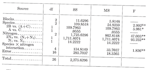
We conclude that species B is poorer than A or C and that there is no difference in growth between A and C. We also conclude that nitrogen adversely affected growth and that 100 pounds was about as bad as 200 pounds. The nitrogen effect was about the same for all species (i.e., no interaction).
It is worth repeating that the comparisons to be made in an analysis should, whenever possible, be planned and specified prior to an examination of the data. A good procedure is to outline the analysis, putting in all the items that are to appear in the first two columns (source and df) of the table. In the above tabulation, last column. * means significant at the 0.05 level. As in the previous table, ** means significant at the 0.01 level, and NS means nonsignificant.
The factorial experiment, it will be noted, is not an experimental design. It is, instead, a way of selecting treatments; given two or more factors each at two or more levels, ,th treatments are all possible combinations of the levels of each factor. If we have three factors with the first at four levels, the second at two levels, and the third at three levels, we will have \(4*2*3=24\) factorial combinations or treatments. Factorial experiments maay be conducted on any of the standard designs. The randomized block and split plot design are the most common for factorial experiments in forest research.
7.6 The Split Plot Design
When two or more types of treatment are applied in factorial combinations, it may be that one type can be applied on relatively small plots while the other type is best applied to larger plots. Rather than make all plots of the size needed for the second type, a split-plot design can be employed. In this design, the major (large-plot) treatments are applied to a number of plots with replication accomplished through any of the common designs (such as complete randomization, randomized blocks, Latin square). Each major plot is then split into a number of subplots, equal to the number of minor (small-plot) treatments. Minor treatments are assigned at random to subplots within each major plot.
As an example, a test was to be made of direct seeding of loblolly pine at six different dates, on burned and unburned seedbeds. To get typical burn effects, major plots 6 acres in size were selected. There were to be four replications of major treatments in randomized blocks. Each major plot was divided into six 1-acre subplots for seeding at six dates. The field layout was somewhat as follows (blocks denoted by Roman numerals, burning treatment by capital letters, date of seeding by small letters):
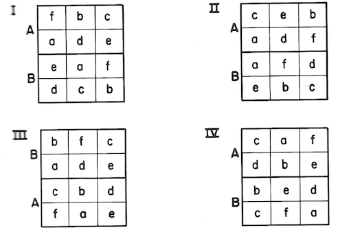
One pound of seed was sowed on each 1-acre subplots. Seedling counts were made at the end of the first growing season. Results were as follows:
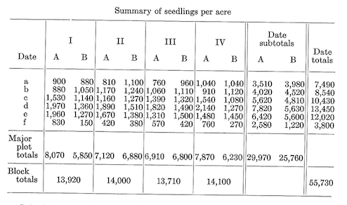
Calculations.-The correction term and total sum of squares are calculated using the 48 subplot values. \[C.T.=\frac {(\text {Grand total of all subplots})^2}{\text {Total number of subplots}}=\frac {55,730^2}{48}=64,704,852\]
\[\text {Total }SS_{47df}=\sum^{48}(\text {Subplot values}^2)-C.T.=9,339,648\]
Before partitioning the total sum of squares into its components it may be instructive to ignore subplots for the moment, and examine the major plot phase of the study. The major phase can be viewed as a straight randomized block design with two burning treatment in ech of four blocks. The analysis would be:
| Source | df |
|---|---|
| Blocks | 3 |
| Burning | 1 |
| Error (major plots) | 3 |
| Major plots | 7 |
Now, looking at the subplots, we can think of the major plots as blocks. From this standpoint we would have a randomized block design with six dates of treatment in each of eight blocks (major plots) for which the analysis is:
| Source | df |
|---|---|
| Major plots | 7 |
| Dates | 5 |
| Remainder | 35 |
| Subplots (=Total) | 47 |
In this analysis, the remainder is made up of two components. One of these is the burning-date interaction, with five dfs. The rest with 30 dfs is called the subplot error. Thus, the complete breakdown of the split-plot design is:
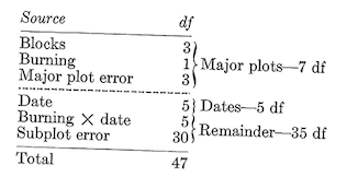
The various sums of squares are obtained in an analogous manner. We first compute: \[\text {Major plot SS}_{7df}=\frac {\sum^8(\text {Major plot totals}^2)}{\text {Number of subplots per major plot}}-C.T.=\frac {8070^2+...+6230^2}{6}-C.T.=647,498\]
\[\text {Block SS}_{3df}=\frac {\sum^4 (\text {Block totals}^2)}{\text {Subplots per block}}-C.T.=\frac {13,920^2+...+14,100^2}{12}-C.T.=6,856\]
\[\text {Burning SS}_{1df}=\frac {\sum^2(\text {Burning treatment totals}^2)}{\text {Subplots per burning treatment}}-C.T.=\frac {29,970^2+25,760^2}{24}-C.T.=369,252\] \[\text {Major plot error SS}_{3df}=\text {Major plot SS}_{7df}-\text {Block SS}_{3df}-\text {Burning SS}_{1df}=271,390\]
\[\text {Subplot SS}_{40df}=\text {Total SS}_{47df}-\text {Major plot SS}_{7df}=8,692,150\] \[\text {Date SS}_{5df}=\frac {\sum^6 (\text {Date totals}^2}{\text {Subplots per date}}-C.T.=\frac {7490^2+...+3800^2}{8}-C.T.=7,500,086\]
Date burning SS: To get the sum of squares for the interaction between date and burning we resort to a factorial experiment device-the two-way table of the treatment combination totals.
| Burning | a | b | c | d | e | f | Burning subtotals |
|---|---|---|---|---|---|---|---|
| A | 3,510 | 4,020 | 5,620 | 7,820 | 6,420 | 2,580 | 29,970 |
| B | 3,980 | 4,520 | 4,810 | 5,630 | 5,600 | 1,220 | 25,760 |
| Date subtotals | 7,490 | 8,540 | 10,430 | 13,450 | 12,020 | 3,800 | 55,730 |
\[\text {Date-burning subclass SS}_{11df}=\frac {\sum^{12}(\text {Date-burning combination totals}^2)}{\text {Subplots per date-burning combination}}-C.T.=\frac {3,510^2+...+1,220^2}{4}-C.T.=8,555,723\]
\[\text {Date-burning interaction SS}_{5df}=\text {Date-burning subclass SS}_{11df}=\text {Date SS}_{5df}-\text {Burning SS}_{1df}=686,385\]
\[\text {Subplot error SS}_{30df}=\text {Subplot SS}_{40df}-\text {Date SS}_{5df}-\text {Date-burning interaction SS}_{5df}=505,679\] Thus the completed analysis table is:
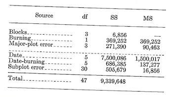
The \(F\) test for burning is \[f_{1/3df}=\frac {\text {Burning MS}}{\text {Major-plot error MS}}=\frac {369,252}{90,463}=4.082, \text {not significant at the 0.05 level}.\]
For dates, \[F_{5/30df}=\frac {\text {Date MS}}{\text {Subplot error MS}}=\frac {1,500,017}{16,856}=88.99, \text {significant at the 0.01 level}.\]
And for the date-burning interaction, \[F_{5/30df}=\frac {\text {Date-burning MS}}{\text {Subplot error MS}}=\frac {137,277}{16,856}=8.14, \text {significant at the 0.01 level}.\]
Note that the major-plot error is used to test the sources above the dashed line while the subplot error is for the sources below the line. Because the subplot error is a measure of random variation within major plots it will usually be smaller than the major-plot error, which is a measure of the random variation between major plots. In addition to being smaller, the subplot error will generally have more degrees of freedom than the major-plot error, and for these reasons the sources below the dashed line will usually be tested with greater sensitivity than the sources above the line. This fact is important; in planing a split-plot experi ment the designer should try to get the items of greatest interest below the line rather then above. Rarely will the major-plot error be appreciably smaller than the subplot error. If it is, the conduct of the study and the computations should be carefully examined.
Subplots can also be split–If desired, the subplots can also be split for a third level of treatment, producing a split-split-plot design. The calculations follow the same general pattern but are more involved. A split-split-plot design has three separate error terms.
Comparisons among means in a split-plot design–For comparisons among major-or subplot treatments, \(F\) tests with a single degree of freedom may be made in the usual manner. Comparisons among major-plot treatments should be tested against the major-plot error mean square, while subplot treatment comparisons are tested against the subplot error. In addition, it is sometimes desirable to compare the means of two treatment combinations. This can get tricky, for the variation among such common cases are discussed below.
In general, the \(t\) test for comparing two equally replicated treatment means is: \[t=\frac {\text {Mean difference}}{\text {Standard error of the mean difference}}=\frac {\bar D}{s_\bar D}\]
- For the difference between two major-treatment means: \[s_\bar D=\sqrt {{2(\text {Major-plot error MS})} \over (m)(R)};\text {t has df equal to the df for the major-plot error}.\]
where:
$R =
$m =
- For the difference between two minor-treatment means: \[s_{\bar D}=\sqrt {{2(\text {Subplot error MS})} \over (R)(M)};\text {t has df equal to the df for subplot error} \]
where:
\(M = \text {Number of major-plot treatments}.\)
For the difference between two minor treatments within a single major treatment: \[s_{\bar D}=\sqrt {{2(\text {Subplot error MS})} \over (R)};\text {df for t=df for the subplot error}\]
For the difference between the means of two major treatments at a single level of a minor treatment, or between the means of two major treatments at different levels of a minor treatment: \[s_\bar D=\sqrt {2[\frac {(m-1)(\text {Subplot error MS})+\text {Major-plot error MS}}{(m)(R)}]}\]
In this case \(t\) will not follow the \(t\) distribution. A close approximation to the value of \(t\) required for significance at the \(\alpha\) level is given by: \[t=\frac {(m-1)(\text {Subplot error MS})t_m+(\text {Major-plot error MS})t_M}{(m-1)(\text {Subplot error MS})+(\text {Major-plot error MS})}\]
where:
\(t_m\)=Tabular value of \(t\) at the \(\alpha\) level for df equal to the df for the subplot error.
\(t_M\)=Tabular value of \(t\) at the \(\alpha\) level for df equal to the df for the major-plot error.
Other symbols are as previously defined.
7.7 Missing Plots
A mathematician who had developed a complex electronic computer program for analyzing a wide variety of experimental designs was asked how he handled missing plots. His disdainful reply was, “We tell our research workers not to have missing plots.”
This is good advice. But it is sometimes hard to follow, and particularly so in forest research, where close control over experimental material is difficult and studies may run for several years.
The likelihood of plots being lost during the course of a study should be considered when selecting an experimental design. Lost plots are least troublesome in the simple designs. For this reason, complete randomization and randomized blocks may be preferable to the more intricate designs when missing data can be expected.
In the complete randomization design, loss of one or more plots causes no computational difficulties. The analysis is made as though the missing plots never existed. Of course, a degree of freedom will be lost from the total and error terms for each missing plot and the sensitivity of the test will be reduced. If missing plots are likely, the number of replications should be increased accordingly.
In the randomized block design, completion of the analysis will usually require an estimate of the values for the missing plots. A single missing value can be estimated by: \[X=\frac {bB+tT-G}{(b-1)(t-1)}\]
where:
\(b\)=Number of blocks \(t\)=Number of treatments \(B\)=Total of all other units in the block with a missing plot \(T\)=Total of all other units that received the same treatment as the missing plot \(G\)=Total of all observed units
If more than one plot is missing, the customary procedure is to insert guessed values for all but one of the missing units, which is then estimated by the above formula. This estimate is used in obtaining an estimated value for one of the guessed plots, and so on through each missing unit. Then the process is repeated until the new approximations differ little from the previous estimates.
The estimated values are now applied in the usual analysis-of-variance calculations. For each missing unit one degree of freedom is deducted from the total and from the error term.
A similar procedure is used with the Latin square design, but the formula for a missing plot is: \[X=\frac {r(R+C+T)-2G}{(r-1)(r-2)}\]
where:
\(r\)=Number of rows \(R\)=Total of all observed units in the row with the missing plot \(C\)=Total of all observed units in the column with the missing plot \(T\)=Total of all observed units in the missing plot treatment \(G\)=Grand total of all observed units
With the split-plot design, missing plots can cause trouble. A single missing subplot value can be estimated by the equation: \[X=\frac {rP+m(T_{ij})-(T_i)}{(r-1)(m-1)}\]
where:
\(r\)=Number of replications of major-plot treatments \(P\)=Total of all observed subplots in the major plot having a missing subplot \(m\)=Number of subplot treatments \(T_{ij}\)=Total of all subplots having the same treatment combination as the missing unit \(T_i\)=Total of all subplots having the same major-plot treatment as the missing unit
For more than one missing subplot the iterative process described for randomized blocks must be used. In the analysis, one df will be deducted from the total and subplot error terms for each missing subplot.
When the data for missing plots are estimated, the treatment mean square for all designs is biased upwards. If the proportion of missing plots is small, the bias can usually be ignored. Where the proportion is large, adjustments can be made as described in the standard references on experimental designs.