Chapter 8 Regression

8.1 Simple Linear Regression

A forester had an idea that he could tell how well a loblolly pine was growing from the volume of the crown. Very simple: big crown-good growth, small crown-poor growth. But he couldn’t say how big and how good, or how small and how poor. What he needed was regression analysis: it would enable him to express a relationship between tree growth and crown volume in an equation. Given a certain crown volume, he could use the equation to predict what the tree growth was.

To gather data, he ran parallel survey lines across a large tract that was representative of the area in which he was interested. The lines were 5 chains apart. At each 2-chain mark along the lines, he measured the nearest loblolly pine of at least 5.6 inches d.b.h. for crown volume and basal area growth over the past 10 years.

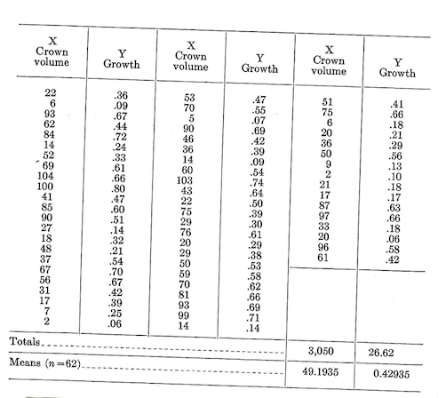
A portion of the data is printed below to illustrate the methods of calculation. Crown volume in hundreds of cubic feet is labeled \(X\) and basal area growth in square feet is labeled \(Y\). Now, what can we tell the forester about the relationship.

Often, the first step is to plot the field data on coordinate paper (fig.1). This is done to provide some visual evidence of whether the two variables are related. If there is a simple relationship, the plotted points will tend to form a pattern (a straight line or curve). If the relationship is very strong, the pattern will generally be distinct. If the relationship is weak, the points will be more spread out and the pattern less definite. If the points appear to fall pretty much at random, there may be no simple relationship or one that is so very poor as to make it a waste of time to fit any regression.

The type of pattern (straight line, parabolic curve, exponential curve, etc.) will influence the regression model to be fitted. In this particular case, we will assume a simple straight-line relationship.

After selecting the model to be fitted, the next step will be to calculate the corrected sums of squares and products. In the following equations, capital letters indicate uncorrected values of the variables; lower-case letters will be used for the corrected values (\(y=Y-\bar Y\)).

The corrected sum of squares for Y: \(\sum y^2=\sum^nY^2-\frac {(\sum^nY)^2}{n}=(0.36^2+0.09^2+...+0.42^2)-\frac {26.62^2}{62}=2.7826\)

The corrected sum of squares for X: \(\sum x^2=\sum X^2-\frac {(\sum X)^2}{n}=(22^2+6^2+...+61^2)-\frac {3,050^2}{62}=59,397.6775\)

The corrected sum of products: \(\sum {xy}=\sum^n (XY)-\frac {(\sum^n X)(\sum^n Y)}{n}=[(22)(0.36)+(6)(0.09)+...+(61)(0.42)]-\frac {(3,050)(26.62)}{62}=354.1477\)

The general form of equation for a straight line is \(Y=a+bX\)

In this equation, a and b are constants or regression coefficients that must be estimated. According to the principle of least squares, the best estimates of these coefficients are: \[b=\frac {\sum {xy}}{\sum x^2}=\frac {354.1477}{59,397.6775}=0.005962\]

\[a=\bar Y-b\bar X=0.42935-(0.005962)(49.1935)-0.13606\] Substituting these estimates in the general equation gives: \[\hat Y=0.13606+0.005962X\]

where \(\hat Y\) is used to indicate that we are dealing with an estimated value of \(Y\).

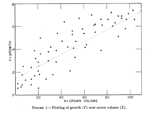
With this equation we can estimate the basal area growth for the past 10 years \((\hat Y)\) from the measurements of the crown volume \(X\).

Because \(Y\) is estimated from a known value of \(X\), it is called the dependent variable and \(X\) the independent variable. In plotting on graph paper, the values of \(Y\) are usually (purely by convention) plotted along the vertical axis (ordinate) and the values of \(X\) along the horizontal axis (abscissa).

8.1.1 How Well Does the Regression Line Fit the Data?

A regression line can be thought of as a moving average. It gives an average value of \(Y\) associated with a particular value of \(X\). Of course, some values of \(Y\) will be above the regression line (or moving average) and some below, just as some values of \(Y\) are above or below the general average of \(Y\).

The corrected sum of squares for \(Y\) (i.e., \(\sum y^2\)) estimates the amount of variation of individual values of \(Y\) about the mean value of \(Y\). A regression equation is a statement that part of the observed variation in \(Y\) (estimated by \(\sum y^2\)) is associated with the relationship of \(Y\) to \(X\). The amount of variation in \(Y\) that is associated with the regression on \(X\) is called the reduction or regression sum of squares. \[\text {Reduction SS}=\frac {(\sum {xy})^2}{\sum x^2}=\frac {(354.1477)^2}{(59,397.6775)}=2.1115\]

As noted above, the total variation in \(Y\) is estimated by \(\sum y^2=2.7826\) (as previously calculated).

The part of the total variation in \(Y\) that is not associated with the regression is called the residual sum of squares. It is calculated by: \[\text {Residual SS}=\sum y^2-\text {Reduction SS}=2.7826-2.115=0.6711\]

In analysis of variance, we used the unexplained variation as a standard for resting the amount of variation attributable to treatments. We can do the same in regression. What’s more, the familiar \(F\) test will serve.

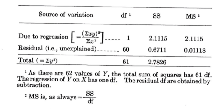
The regression in tested by \[F=\frac {\text {Regression MS}}{\text {Residual MS}}=\frac {2.1115}{0.01118}=188.86\]

As the calculated \(F\) is much greater than tabular \(F_{0.01}\) with 1/60 df , the regression is deemed significant at the 0.01 level.

Before we fitted a regression line to the data, \(Y\) had a certain amount of variation about its mean \((\bar Y)\). Fitting the regression was, in effect, an attempt to explain part of this variation by the linear association of \(Y\) with \(X\). But even after the line had been fitted, some variation was unexplained–that of \(Y\) about the regression line. When we tested the regression line above, we merely showed that the part of the variation in \(Y\) that is explained by the fitted line is significantly greater than the part that the line left unexplained. The test did not show that the line we fitted gives the best possible description of the data (a curved line might be even better). Nor does it mean that we have found the true mathematical relationship between the two variables. There is a dangerous tendency to ascribe more meaning to a fitted regression than is warranted.

It might be noted that the residual sum of square is equal to the sum of the squared deviations of the observed values of \(Y\) from the regression line. That is, \[\text {Residual SS}=\sum (Y-\hat Y)^2=\sum (Y-a-bX)^2\]

The principle of least squares says that they best estimates of the regression coefficients (\(a\) and \(b\)) are those that make this sum of squares a minimum.

8.1.2 Coefficient of Determination

As a measure of how well a regression fits the sample data, we can compute the proportion of the total variation in \(Y\) that is associated with the regression. This ratio is sometimes called the coefficient of determination. \[\text {Coefficient of Determination}={\text {Reduction SS} \over \text {Total SS}}=\frac {2.1115}{2.7826}=0.758823\]

When someone says, “76 percent of the variation in \(Y\) was associated with \(X\),” they mean that the coefficient of determination was 0.76.

The coefficient of determination is equal to the square of the correlation coefficient. \[\frac {\text {Reduction SS}}{\text {Total SS}}=\frac {(\sum xy)^2/\sum x^2}{\sum y^2}=\frac {(\sum xy)^2}{(\sum x^2)(\sum y^2)}=r^2\]

In fact, most present-day users of regression refer to \(r^2\) values rather than to coefficients of determination.

In the older literature, \(1-r^2\) is sometimes called the coefficient of non-determination, and \(\sqrt {1-r^2}\) has been called the alienation index.

8.1.3 Confidence Intervals

Since it is based on sample data, a regression equation is subject to sample variation. Confidence limits on the regression line can be obtained by specifying several values over the range of \(X\) and computing \[\text {Confidence limits}=\hat Y \pm t\sqrt {(\text {Residual MS})(\frac {1}{n}+\frac {(X_0-\bar X)^2}{\sum x^2})}\]

Where:

\(X_0=\) a selected value of \(X\), and degrees of freedom for \(t=df\) for residual MS

In the example we had:

\[\hat Y=0.13606+0.005962X\] \[\text {Residual MS}=0.01118 \text {with 60 dfs}\] \[n=62\]

\[\bar X=49.1935\]

\[\sum x^2=59,397.6775\]

So, if we pick \(X_0=28\) we have \(\hat Y=0.303\), and 95-percent confidence limits

\[=0.303 \pm 2.000 \sqrt {(0.01118)(\frac {1}{62}+\frac {(28-49.1935)^2}{59,397.6775})}=0.270 \text { to } 0.336\]

For other values of \(X_0\) we would get:

\(X_0\)	\(\hat Y\)	95% lower limit	95% upper limit
8	0.184	0.139	0.229
49.1935	0.429	0.402	0.456
70	0.553	0.521	0.585
90	0.672	0.629	0.717

In figure 2 these points have been plotted and connected by smooth curves.

It should be especially noted that these are confidence limits on the regression of \(Y\) on \(X\). They indicate the limits within which the true mean of \(Y\) for a given \(X\) will lie unless a one-in-twenty chance has occurred. The limits do not apply to a single predicted value of \(Y\). The limits within which a single \(Y\) might lie are given by: \[\hat Y \pm t \sqrt {(\text {Residual MS})(1+\frac {1}{n}+\frac {(X_0-\bar X)^2}{\sum x^2})}\]

Assumptions.–In addition to assuming that the relationship of \(Y\) to \(X\) is linear, the above method of fitting assumes that the variance of \(Y\) about the regression line is the same at all levels of \(X\) (the assumption of homogenous variance or homoscedasticity–if you want to impress your friends). The fitting does not assume nor does it require that the variation of \(Y\) about the regression line follows the normal distribution. However, the \(F\) test does assume normality, and so does the use of \(t\) for the computation of confidence limits.

There is also an assumption of independence of the errors (departures from regression) of the sample observations. The validity of this assumption is best insured by selecting the sample units at random. The requirement of independence may not be met if successive observations are made on a single unit or if the units are observed in clusters. For example, a series of observations of tree diameter made by means of a growth band would probably lack independence.

Selecting the sample units so as to get a particular distribution of the \(X\) values does not violate any of the regression assumptions, provided the \(Y\) values are a random sample of all \(Y\)s associated with the selected values of \(X\). Spreading the sample over a wide range of \(X\) values will usually increase the precision with which the regression coefficients are estimated. This device must be used with caution however, for if the \(Y\) values are not random, the regression coefficients and residual mean squares may be improperly estimated.

8.2 Multiple Linear Regression

It frequently happens that a variable \((Y)\) in which we are interested is related to more than one independent variable. If this relationship can be estimated, it may enable us to make more precise predictions of the dependent variable than would be possible by a simple linear regression. This brings us up against multiple regression, which is a little more work but no more complicated than a simple linear regression.

The calculation methods can be illustrated with the following set of hypothetical data from a study relating the growth of even-aged loblolly-shortleaf pine stands to the total basal area \((X_1)\), the percentage of the basal area in loblolly pine \((X_2)\), and loblolly pine site index \((X_3)\).

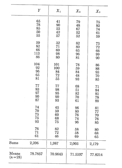
With this data we would like to fit an equation of the form \[Y=a+b_1X_1+b_2X_2+b_3X_3\]

According to the principle of least squares, the best estimates of the \(X\) coefficients can be obtained by solving the set of least squares normal equations.

\(b_1\) equation: \[(\sum x_1^2)b_1+(\sum x_1x_2)b_2+(\sum x_1x_3)b_3=\sum x_1y\] \(b_2\) equation: \[(\sum x_1x_2)b_1+(\sum x_2^2)b_2+(\sum x_2x_3)b_3=\sum x_2y\] \(b_3\) equation: \[(\sum x_1x_3)b_1+(\sum x_2x_3)b_2+(\sum x_3^2)b_3=\sum x_3y\]

where: \[\sum x_ix_j=\sum X_iX_j-\frac {(\sum X_i)(\sum X_j)}{n}\]

Having solved for the \(X\) coefficients (\(b_1,b_2,\text { and }b_3\)), we obtain the constant term by solving \[a=\bar Y-b_1\bar X_1-b_2\bar X_2-b_3\bar X_3\]

Derivation of the least squares normal equations requires a knowledge of differential calculus. However, for the general linear model with a constant term \[Y=a+b_1X_1+b_2X_2+...+b_kX_k\]

the normal equations can be written quite mechanically once their pattern has been recognized. Every term in the first row contains an \(x_1\), every term in the second row an \(x_2\), and so forth down to the \(k^{th}\) row, every term of which will have and \(x_k\). Similarly, every t$erm in the first column has an \(x_1\) and a \(b_1\), every term in the second column has an \(x_2\) and a \(b_2\), and so on through the \(k^{th}\) column, every term of which has an \(x_k\) and a \(b_k\). On the right side of the equations, each term has a \(y\) times the \(x\) that is appropriate for a particular row. So, for the general linear model given above, the normal equations are:

\(b_1\) equation: \[(\sum x_1^2)b_1+(\sum x_1x_2)b_2+(\sum x_1x_3)b_3+...+(\sum x_1x_k)b_k=\sum x_1y\] \(b_2\) equation: \[(\sum x_1x_2)b_1+(\sum x_2^2)b_2+(\sum x_2x_3)b_3+...+(\sum x_2x_k)b_k=\sum x_2y\] \(b_3\) equation: \[(\sum x_1x_3)b_1+(\sum x_2x_3)b_2+(\sum x_3^2)b_3+...+(\sum x_3x_k)b_k=\sum x_3y\]

---

\(b_k\) equation: \[(\sum x_1x_k)b_1+(\sum x_2x_k)b_2+(\sum x_3x_k)b_3+...+(\sum x_k^2)b_k=\sum x_ky\]

Given the \(X\) coefficients, the constant term can be computed as \[a=\bar Y-b_1\bar X_1-b_2\bar X_2-...-b_k\bar X_k\]

Note that the normal equations for the general linear model include the solution for the simple linear regression \[(\sum x_1^2)b_1=\sum x_1y\]

Hence, \[b_1=(\sum x_1y)/\sum x_1^2 \text { as previously given}\].

In fact, all of this section on multiple regression can be applied to the simple linear regression as a special case.

The corrected sums of squares and products are computed in the familiar (by now) manner:

\[\sum y^2=\sum Y^2-\frac {(\sum Y^2)}{n}=(65^2+...+61^2)-\frac {(2206)^2}{28}=5,974.7143\]

\[\sum x_1^2=\sum X_1^2-\frac {(\sum X_1)^2}{n}=(41^2+...+46^2)-\frac {(1987)^2}{28}=11,436.9643\]

\[\sum x_1y=\sum X_1Y-\frac {(\sum X_1)(\sum Y)}{n}=(41)(65)+...+(46)(61)-\frac {(1,987)(2,206)}{28}=6,428.7858\]

Similarly,

\(\sum x_1x_2=-1,171.4642\)

\(\sum x_1x_3=3,458.8215\)

\(\sum x_2^2=5,998.9643\)

\(\sum x_2x_3=1,789.6786\)

\(\sum x_2y=2,632.2143\)

\(\sum x_3^2=2,606.1072\)

\(\sum x_3y=3,327.9286\)

Putting these values in the normal equations gives:

\[11,436.9643b_1-1,171.4642b_2+3,458.8215b_3=6,428.7858\]

\[-1,171.4642b_1+5,998.9643b_2+1,789.6786b_3=2,632.2143\]

\[3,458.8215b_1+1,789.6786b_2+2,606.1072b_3=3,327.9286\]

These equations can be solved by any of the standard procedures for simultaneous equations. One approach (applied to the above equations) is as follows:

1. Divide through each equation by the numerical coefficient of \(b_1\).

\[b_1-0.102,427,897b_2+0.302,424,788b_3=0.562,105,960\]

\[b_1-5.120,911,334b_2-1.527,727949b_3=-2.246,943,867\]

\[b_1+0.517,424,389b_2+0.753,466,809b_3=0.962,156,792\]

2. Subtract the second equation from the first and the third from the first so as to leave tow equations in \(b_2\) and \(b_3\).

\[5.018,483,437b_2+1.830,152,737b_3=2.809,049,827\]

\[-0.619,852,286b_2-0.451,042,021b_3=-0.400,050,832\]

3. Divide through each equation by the numerical coefficient of \(b_2\).

\[b_2+0.364,682,430b_3=0.559,740,779\]

\[b_2+0.727,660,494b_3=0.645,397,042\]

4. Subtract the second of these equations from the first, leaving one equation in \(b_3\).

\[-0.362,978,064b_3=-0.085,656,263\]

5. Solve for \(b_3\)

\[b_3=\frac {-0.085,656,263}{-0.362,978,064}=0.235,981,927\]

6. Substitute this value of \(b_3\) in one of the equations (say the first) of step 3 and solve for \(b_2\).

\[b_2+(0.364,682,430)(0.235,981,927)=0.559,740,779\]

\[b_2=0.473,682,316\]

7. Substitute the solutions for \(b_2\) and \(b_3\) in one of the equations (say the first) of step 1, and solve for \(b_1\).

\[b_1(0.102,427,897)(0.473,682,316)+(0.302,424,788)(0.235,981,927)=0.562,105,960\]

\[b_1=0.539,257,459\]

8. As a check, add up the original normal equations and substitute the solutions for \(b_1, b_2, b_3\).

\[13,724.3216b_1+6,617.1787b_2+7,854.6073b_3=12,388.9287\]

\[12,388.92869 \text { approximately equal to }12, 388.9287, \text { check}\]

Given the values of \(b_1, b_2, b_3\) we can now compute \[a=\bar Y-b_1\bar X_1-b_2\bar X_2-b_3\bar X_3=-11,7320\]

Thus, after rounding of the coefficients, the regression equation is \[\hat Y=-11.732+0.539X_1+0.474X_2+0.236X_3\]

It should be noted that in solving the normal equations more digits have been carried than would be justified by the rules for number of significant digits. Unless this is done the rounding errors may make it difficult to check the computations.

8.2.1 Tests of Significance

To test the significance of the fitted regression, the outline for the analysis of variance is

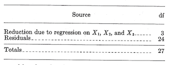
The degrees of freedom for the total are equal to the number of observations minus 1. The total sum of squares is \[\text {Total SS}=\sum y^2=5,974.7143\]

The degrees of freedom for the reduction are equal to the number of independent variables fitted, in this case 3. The reduction sum of squares for any least squares regression is \[\text {Reduction SS}=\sum (\text {estimated coefficients})(\text {right side of their normal equations})\]

In this example there are three coefficients estimated by the normal equations, as so \[\text {Reduction SS}_3df=b_1(\sum x_1y)+b_2(\sum x_2y)+b_3(\sum x_3y)=(0.53926)(6,428.7858)+(0.47368)(2,632.2143)+(0.23598)(3,327.9286)=5,498.9389\]

The residual df and sum of squares are obtained by subtraction. This the analysis becomes:

To test the regression we compute \[F_{3/24df}=\frac {1,832.9796}{19.8240}=92.46\]

which is significant at the 0.01 level.

Often we will want to test individual terms of the regression. In the previous example we might want to test the hypothesis that the true value of \(b_3\) is zero. This would be equivalent to testing whether the variable \(X_3\) makes any contribution to the prediction of Y. If we decide what \(b_3\) may be equal to zero, we might rewrite the equation in terms of \(X_1\) and \(X_2\). Similarly, we could test the hypothesis that \(b_1\) and \(b_3\) are both equal to zero.

To test the contribution of any set of the independent variables in the presence of the remaining variables:

1. Fit all independent variables and compute the reduction and residual sums of squares.

2. Fit a new regression that includes only the variables not being tested. Compute the reduction due to this regression.

3. The reduction obtained in the first step minus the reduction in the second step is the gain due to the variables being tested.

4. The mean square for the gain (step 3) is tested against the residual mean square for the first step.

Two examples will illustrate the procedure:

I. Test \(X_1\) and \(X_2\) in the presence of \(X_3\).

1. The reduction due to \(X_1, X_2, X_3\) is 5,498.9389 with 3 df. The residual is 475.7754 with 24 degrees of freedom (from previous example).

2. For fitting \(X_3\) alone, the normal equation is \[(\sum x_3^2)b_3=(\sum x_2y)\]

or \[2,606.1072b_3=3,327.9286\]

\[b_3=1.27697\]

The reduction due to \(X_3\) alone is \[\text {Red. SS}=b_3(\sum x_3y)=1.27697(3,3327.9286)=4,249.6650 \text { with 1 df}.\]

3. The gain due to \(X_1\) and \(X_2\) after \(X_3\) is \[\text {Gain SS}=\text {Reduction due to }X_1, X_2, X_3-\text {reduction due to }X_3\text { alone}\]

\[5,498.9389-4,249.6650\]

\[1,249.2739 \text { with (3-1)=2 df}\]

4. Then \[F_{2/24df}=\frac {\text {Gain MS}}{\text {Residual MS}}=\frac {624.63695}{19.8240}=31.51, \text { significant at the 0.01 level}.\]

This test is usually presented in the analysis of variance form:

2. Test \(X_2\) in the presence of \(X_1\) and \(X_3\)

The normal equations for fitting \(X_1\) and \(X_3\) are \[(\sum x_1^2)b_1+(\sum x_1x_3)b_3=\sum x_1y\]

\[(\sum x_1x_3)b_1+(\sum x_3^2)b_3=\sum x_3y\]

or

\[11,436.9643b_1+3,458.8215b_3=6,428.7858\]

\[3,458.8215b_1+2,606.1072b_3=3,327.9286\]

The solutions are \[b_1=0.29387\]

\[b_3=0.88695\]

The reduction sum of squares is \[\text {Reduction SS}=b_1(\sum x_1y)+b_3(\sum x_3y)=(0.29387)(6,428.7858)_(0.88695)(3,327.9286)=4,840.9336, \text { with 2 df}\]

The analysis is:

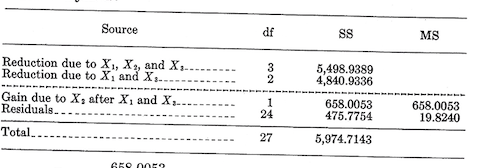
\[F_{1/24df}=\frac {658.0053}{19.8240}=33.19, \text { significant at the 0.01 level}.\]

8.2.2 Coefficient of Multiple Determination

As a measure of how well the regression fits the data, it is customary to compute the ratio of the reduction sum of squares to the total sum of squares. This ratio is symbolized by \(R^2\) and is sometimes called the coefficient of determination: \[R^2=\frac {\text {Reduction SS}}{\text {Total SS}}\]

For the regression of \(Y\) on \(X_1\), \(X_2\), and \(X_3\), \[R^2=\frac {5,498.9389}{5,974.7143}=0.92\]

The \(R^2\) value is usually referred to by saying that a certain percentage (92 in this case) of the variation in \(Y\) is associated with the regression.

The square root (R) of the ratio is called the multiple correlation coefficient.

8.2.3 The c-multipliers

Putting confidence limits on a multiple regression requires computation of the Gauss or c-multipliers. The c-multipliers are the elements of the matrix of corrected sums of squares and products as they appear in the normal equations. Thus, in fitting the regression of \(Y\) on \(X_1\), \(X_2\), and \(X_3\) the matrix of corrected sums of squares and products is:

The inverse of this matrix is:

The matrix of c-multipliers is symmetric, and therefore \(c_{12}=c_{21},c_{13}=c_{31}, etc.\)

The procedure for calculating the c-multipliers will not be given here. Those who are interested can refer to one of the standard statistical textbooks such as Goulden or Snedecor. However, because the c-multipliers are the output of many electronic computer programs, some of their applications will be described.

One of the important uses is in the calculation of confidence limits on the mean value of \(Y\) (i.e., regression \(Y\)) associated with a specified set of \(X\) values. The general equation for \(k\) independent variables is: \[\text {confidence limits}=\hat Y \pm t\sqrt{\text {Residual MS}(\frac {1}{n}+\sum_i\sum_j c_{ij}(X_1-\bar X_i)(X_j-\bar X_j))}\]

where:

\(i\) and \(j\) each go from 1 to \(k\)

\(t\) has df equal to the degrees of freedom for the residual mean square.

In the example, if we specify \(X_1=80.9643\), \(X_2=66.5357\), and \(X_3=76.8214\), then \(\hat Y=81.576\) and the 95-percent confidence limits are:

\[81.576 \pm 2.064{\sqrt{19.8240[\frac{1}{28}+c_{11}(80.9643-\bar X_1)^2+c_{22}(66.5357-\bar X_2)^2+c_{33}(76.8214-\bar X_3)^2+2C_{12}(80.9643-\bar X_1)(66.5357-\bar X_2)+2c_{13}(80.9643-\bar X_1)(76.8214-\bar X_{3})+2c_{23}(66.5357-\bar X_2)(76.8214-\bar X_3)]}}\]

\[=81.576 \pm 2.064{\sqrt{19.8240[\frac{1}{28}+0.019,948,390]}}\]

\[=79.41 \text { to }83.74\]

Note that each cross-product term such as \(c_{13}(X_1-\bar X_1)(X_3-\bar X_3)\) and \(c_{31}(X_3-\bar X_3)(X_1-\bar X_1)\). As previously noted, the matrix of c-multipliers is symmetric, so that \(c_{13}=c_{31}\); hence we can combine these two terms to get \(2c_{13}(X_1-\bar X_1)(X_3-\bar X_3).\)

For the confidence limits on a single predicted value of \(Y\) (as opposed to mean \(Y\)) associated with a specified set of \(X\) values the equation is \[\hat Y \pm t\sqrt {\text {Residual MS}[1+\frac {1}{n}+\sum_i \sum_j c_{ij}(X_i-\bar X_i)(X_j-\bar X_j)]}\]

With the above set of \(X\) values these limits would be 72.13 to 91.02

The c-multipliers may also be used to calculate the estimated regression coefficients. The general equation is \[b_j=\sum_i c_{ji}(\sum x_iy)\]

where:

\(\sum x_iy=\text {The right hand side of the } i^{th} \text { normal equation}\)

\((i=1,...,k)\).

To illustrate, \(b_2\) in the previous example would be calculated as: \[b_2=c_{21}(\sum x_1y)+c_{22}(\sum x_2y)+c_{23}(\sum x_3y)\]

\[=0.000,176,649(6,428.7858)+0.000,340,994(2,632.2143)-0.000,468,616(3,327.9286)\]

\[=0.47369 \text { as before (except for rounding errors)}\]

The regression coefficients are sample estimates and are, of course, subject to sampling variation. This means that any regression coefficient has a standard error and any pair of coefficients will have a covariance. The standard error of a regression coefficient is estimated by \[\text {Standard Error of }b_j=\sqrt {c_{jj}(\text {Residual MS})}\]

Hence,

\[\text {Variance of b}_j=c_{jj}(\text {Residual MS}).\]

The covariance of any two coefficients is \[\text {Covariance of }b_i \text { and }b_j=c_{ij}(\text {Residual MS}).\]

The variance and covariance equations permit testing various hypotheses about the regression coefficients by means of a \(t\) test in the general form \[t=\frac {\Theta-\Theta}{\sqrt {\text {Variance of }\Theta}}\]

where:

\(\Theta=\) Any linear function of the estimated coefficients \(\Theta=\) Hypothesized value of the function.

In the discussion of the analysis of variance we tested the contribution of \(X_2\) in the presence of \(X_1\) and \(X_3\) (obtaining \(F=33.19\)). This is actually equivalent to testing the hypothesis that in the model \(Y=a+b_1X_1+b_2X_2+b_3X_3\) the true value of \(b_2\) is zero. The \(t\) test of this hypothesis is as follows: \[t=\frac {b_2-0}{\sqrt {\text {Variance of }b_2}}=\frac {b_2}{c_{22}(\text {Residual MS})}=\frac {0.47368}{0.000,340,994(19.8240)}=5.761, \text { with 24 df =df for Residual MS}\]

Note that \(t^2=33.19=\) the \(F\) value obtained in testing this same hypothesis.

It is also possible to test the hypothesis that a coefficient has some value other than zero or that a linear function of the coefficients has some specified value. For example, if there were some reason for believing that \(b_1=2b_3\) or \(b_1-2b_3=0,\) this hypothesis could be tested by \[t=\frac {b_1-2b_3}{\sqrt {\text {Variance of } (b_1-2b_3)}}\]

Referring to the section on the variance of a linear function, we find that:

\[\text {Variance of }(b_1-2b_3)=\text {Variance of }b_1+4(\text {variance of }b_3)-4(\text {covariance of }b_1 \text { and } b_3)\]

\[=(c_{11}+4c_{33}-4c_{13})(\text {Residual MS})=19.8240[(0.000,237,573)+4(0.001,285,000)-4(-0.000,436,615)]\]

\[=0.141,226,830\]

Then, \[t_{24df}=\frac {0.53926-2(0.23598)}{\sqrt {0.141,226,830}}=\frac {0.06730}{0.37580}=0.179\]

The hypothesis would not be rejected at the 0.05 level.

Assumptions.–The assumptions underlying these methods of fitting a multiple regression are the same as those for a simple linear regression: equal variance of \(Y\) at all combinations of \(X\) values and independence of the errors (i.e., departures from regression) of the sample observations. Application of the \(F\) or \(t\) distributions (for testing or setting confidence limits) requires the further assumption of normality.

The reader is again warned against inferring more than is actually implied by a regression equation and analysis. For one thing, no matter how well a particular equation may fit a set of data, it is only a mathematical approximation of the relationship between a dependent and a set of independent variables. IT should not be construed as representing a biological or physical law. Nor does it prove the existence of a cause and effect relationship. It is merely a convenient way of describing an observed association.

Tests of significance must also be interpreted with caution. A significant \(F\) or \(t\) test means that the estimated values of the regression coefficients differ from the hypothesized values (usually zero) by more than would expected by chance. Even though a regression is highly significant, the predicted values may not be very close to the actual (look at the standard errors). Conversely, the fact that a particular variable (say \(X_j\)) is not significantly related to \(Y\) does not necessarily mean that a relationship is lacking. Perhaps the test was insensitive or we did not select the proper model to represent the relationship.

Regression analysis is a very useful technique, but it does not relieve the research worker of the responsibility for thinking.

8.3 Curvilinear Regressions and Interactions

Curves.–Many forms of curvilinear relationships can be fitted by the regression methods that have been described in the previous sections.

If the relationship between height and age is assumed to be hyperbolic so that

\[Height=a+\frac {b}{Age}\]

then we could let \(Y=Height\) and \(X_1=1/Age\) and fit \[Y=a+b_1X_1\]

Similarly, if the relationship between \(Y\) and \(X\) is quadratic \[Y=a+bX+cX^2\]

we can let \(X=X_1\) and \(X_2=X^2\) and fit \[Y=a+b_1X_1+b_2X_2\]

Functions such as \[Y=aX^b\]

\[Y=a(b^X)\]

\[10^Y=aX^b\]

which are nonlinear in the coefficients can sometimes be made linear by a logarithmic transformation. The equation \[Y=aX^b\]

would become \[\text {log }Y=\text {log a}+b(\text {log X})\]

which could be fitted by \[Y'=a'+b_1X_1\]

where

\[Y'=\text {log Y, and}\]

\[X_1=\text {log X}.\] The second equation transforms to \[\text {log Y}=\text {log a}+(\text {log b})X\]

The third becomes

\[Y=\text {log a}+b(\text {log X})\]

Both can be fitted by the linear model.

In making these transformations the effect on the assumption of homogeneous variance must be considered. If \(Y\) has homogeneous variance, log \(Y\) probably will not have–and vice versa.

Some curvilinear models cannot be fitted by the methods that have been described. Some examples are \[Y=a+b^X\]

\[Y=a(X-b)^2\]

\[Y=a(X_1-b)(X_2-c)\]

Fitting these models requires more cumbersome procedures.

Interactions.–Suppose that there is a simple linear relationship between \(Y\) and \(X_1\). If the slope (b) of this relationship varies, depending on the level of some other independent variable (\(X_2\)), \(X_1\) and \(X_2\) are said to interact. Such interactions can sometimes be handled by introducing interaction variables.

To illustrate, suppose that we know that there is a linear relationship between \(Y\) and \(X_1\).

\[Y=a+bX_1\]

Suppose further that we known or suspect that the slope (b) varies linearly with \(Z\) \[b=a'+b'Z\]

This implies the relationship \[Y=a+(a'b'Z)X_1\]

or \[Y=a+a'X_1+b'X_1Z\]

which can be fitted by \[Y=a+b_1X_1+b_2X_2\]

where \(X_2=X_1Z\), an interaction variable.

If the Y-intercept is also a linear function of \(Z\), then \[a=a"+b"Z\]

and the form of relationship is \[Y=a"+b"Z+a'X_1+b'X_1Z\]

which could be fitted by \[Y=a+b_1X_1+b_2X_2+b_3X_3\]

where \(X_2=Z\), and \[X_3=X_1Z\].

8.4 Group Regressions

Linear regressions of \(Y\) on \(X\) were fitted for each of two groups. The basic data and fitted regressions were:

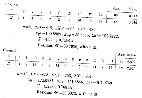
Now we might ask, are these really different regressions? Or could the data be combined to produce a single regression that would be applicable to both groups? If there is no significant difference between the residual mean squares for the two groups (this matter may be determined by Bartlett’s test, page 22), the test described below helps to answer the question.

Testing for the common regressions.–Simple linear regressions may differ either in their slope or in their level. In testing for common regressions the procedure is to test first for common slopes. If the slopes differ significantly, the regressions are different and no further testing is needed. If the slopes are not significantly different, the difference in level is tested. The analysis table is:

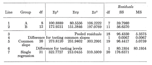
The first two lines in this table contain the basic data for the two groups. To the left are the total df for the groups (8 for \(A\) and 12 for \(B\)). In the center are the corrected sums of squares and products. The right side of the table gives the residual sum of squares and df. Since only simple linear regressions have been fitted, the residual df for each group are on less than the total df. The residual sum of squares is obtained by first computing the reduction sum of squares for each group. \[\text {Reduction SS}=\frac {(\sum xy)^2}{\sum x^2}\]

This reduction is then subtracted from the total sum of squares (\(\sum y^2\)) to give the residuals.

Line 3 is obtained by pooling the residual df and residual sums of squares for the groups. Dividing the pooled sum of squares by the pooled df gives the pooled mean square.

The left side and center of line 5 (we will skip line 4 for the moment) is obtained by pooling the total df and the corrected sums of squares and products for the groups. These are the values that are obtained under the assumptions of no difference in the slopes of the group regressions. If the assumption is wrong, the residuals about this common slope regression will be considerably larger than the mean square residual about the separate regressions. The residual df and sum of squares are obtained by fitting a straight line to this pooled data. The residual df are, of course, one less than the total df. The residual sum of squares is, as usual, \[\text {Residual SS}=273.8120-\frac {(231.9402)^2}{303.2991}=96.4417\]

Now, the difference between thee residuals (line 4=line 5-line 3) provides a test of the hypothesis of common slopes. The error term for this test is the pooled mean square from line 3. \[\text {Test of common slopes:} F_{1/18df}=\frac {0.0067}{5.3575}\]

The difference is not significant.

If the slopes differed significantly, the groups would have different regressions, and we would stop here. Since the slopes did not differe, we now go on to test for a difference in the levels of the regression.

Line 7 is what we would have if we ignored the groups entirely, lumped all the original observations together, and fitted a single linear regression. The combined data are as follows:

\[n=(9+13)=22 (\text {so the df for total}=21)\]

\[\sum Y=(82+79)=161, \sum Y^2=(848+653)=1,501\]

\[\sum y^2=1,501-\frac {(161^2)}{22}=322.7727\]

\[\sum X=(58+99)=157, \sum X^2=(480+951)=1,431\]

\[\sum x^2=1,431-\frac {(157)^2}{22}=310.5909\]

\[\sum XY=(609+753)=1,362, \sum xy=1,362-\frac {(157)(161)}{22}=213.0455\]

From this we obtain the residual values on the right side of line 7.

\[\text {Residual SS}=322.7727-\frac {(213.0455)^2}{310.5909}=176.6371\]

If there is a real difference among the levels of the groups, the residuals about this single regression will be considerably larger than the mean square residual about the regression that assumed the same slopes but different levels. This difference (line 6=line 7-line 5) is tested against the residual mean square from line 5.

\[\text {Test of levels:}F_{1/19df}=\frac {80.1954}{5.0759}=15.80\]

As the levels differ significantly, the groups do not have the same regressions.

The test is easily extended to cover several groups, though there may be a problem in finding which groups are likely to have separate regressions and which can be combined. The test can be extended to multiple regressions.

8.5 Analysis of Covariance in a Randomized Block Design

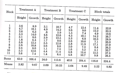
A test was made of the effect of three soil treatments on the height growth of 2-year-old seedlings. Treatments were assigned as random to the three plots within each of the 11 blocks. Each plot was made up of 50 seedlings. Average 5-year height growth was the criterion for evaluating treatments. Initial heights and 5-year growths, all in feet, were:

The analysis of variance of growth is:

Source	df	SS	MS
Blocks	10	132.83
Treatments	2	4.26	2.130
Error	20	68.88	3.444
Total	32	205.97

\[F(\text {for testing treatments})_{2/20df}=\frac {2.130}{3.444}\] \[\text {Not significant at the 0.05 level}\]

There is no evidence of a real difference in growth due to treatments. There is, however, reason to believe that, for young seedlings, growth is affected by initial height. A glance at the block totals seems to suggest that plots with greatest initial height had greatest 5-year growth. The possibility that effects of treatment are being obscured by differences in initial height raises the questions of how the treatments would compare if adjusted for differences in initial heights.

If the relationship between height growth and initial height is linear and if the slope of the regression is the same for all treatments, the test of adjusted treatment means can be made by an analysis of covariance as described below. In this analysis, the growth will be labeled \(Y\) and initial height \(X\).

Computationally the first step is to obtain total, block, treatment, and error sums of squares of \(X\) (\(SS_x\)) and sums of products of \(X\) and \(Y\) (\(SP_{xy}\)), just as has already been done for \(Y\).

For \(X\): \(C.T._x=\frac {116.0^2}{33}=407.76\)

\[\text {Total SS}_x=(3.6^2+...+4.8^2)-C.T._x=73.26\]

\[\text {Block SS}_x=(\frac {11.4^2+...+9.8^2}{3})-C.T._x=54.31\]

\[\text {Treatment SS}_x=\frac {(42.0^2+34.0^2+40.0^2)}{11})-C.T._x=3.15\]

\[\text {Error SS}_x=\text {Total-Block-Treatment}=15.80\]

\[\text {For XY}: C.T._{xy}=\frac {(116.0)(324.4)}{33}=1,140.32\]

\[\text {Total SP}_{xy}=(3.6)(8.9)+...+(4.8)(10.7)-C.T._{xy}=103.99\]

\[\text {Block SP}_{xy}=(\frac {(11.4)(32.0)+...+(9.8)(26.5)}{3})-C.T._{xy}=82.71\]

\[\text {Treatment SP}_{xy}=(\frac {(42.0)(106.4)+(34.0)(113.6)+(40.0)(104.4)}{11})-C.T._{xy}=-3.30\]

\[\text {Error SP}_{xy}=\text {Total-Block-Treatment}=24.58\]

These computed terms are arranged in a manner similar to that for the test of group regressions (which is exactly what the covariance analysis is). One departure is that the total line is put at the top.

On the error line, the residual sum of squares after adjusting for a linear regression is:

\[\text {Residual SS}=SS_y-\frac {(SP_{xy})^2}{SS_x}=68.88-\frac {24.58^2}{15.80}=30.641\]

This sum of squares has 1 df less than the unadjusted sum of squares.

To test treatments we first pool the unadjusted df and sums of squares and products for treatment and error. The residual terms for this pooled line are then computed just as they were for the error line.

Then to test for difference among treatments after adjustment for the regression of growth on initial height, we compute the difference in residuals between the error and the treatment + error lines

	df	SS	MS
Difference for testing adjusted treatments	2	18.603	9.302

The mean square for the difference in residuals is not tested against the residual mean square for error.

\[F_{2/19df}=\frac {9.302}{1.613}=5.77\]

Thus, after adjustment, the difference in treatment means is found to be significant at the 0.05 level. It may also happen that differences that were significant before adjustment are not significant afterwards.

If the independent variable has been affected by treatments, interpretation of a covariance analysis requires careful thinking. The covariance adjustment may have the effect of removing the treatment differences that are being tested. On the other hand, it may be informative to know that treatments are or are not significantly different in spite of the covariance adjustment. The beginner who is uncertain of the interpretations would do well to select as covariates only those that have not been affected by treatments.

The covariance test may be made in a similar manner for any experimental design and, if desired (and justified), adjustment may be made for multiple or curvilinear regressions.

The entire analysis is usually presneted in the following form:

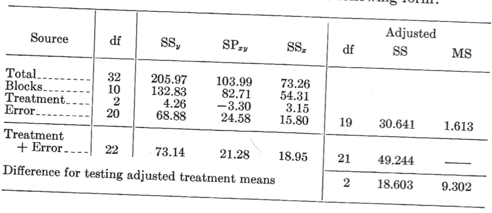
\[\text {Unadjusted treatments}:F_{2/20df}=\frac {2.130}{1.613}. \text { Not significant.}\]

\[\text {Adjusted treatments}:F_{2/19df}=\frac {9.302}{1.613}=5.77. \text { Significant at the 0.05 level}\]

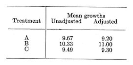
Adjusted means.–If we wish to know what the treatment means are after adjustment for regression, the equation is \[\text {Adjusted }\bar Y_i=\bar Y_i-b(\bar X_i-\bar X)\]

where:

\(\bar Y_i=\text {Unadjusted mean for treatment }i\)

\(b=\text {Coefficient of the linar regression}=\frac {\text {Error SP}_{xy}}{\text {Error SS}_x}\)

\(\bar X_i=\text {Mean of the independent variable for treatment } i\)

\(\bar X=\text {Mean X for all treatments}\)

In the example we had \(\bar X_A=3.82\), \(\bar X_B=3.09\), \(\bar X_C=3.64\), \(\bar X=3.52\), and \(b=\frac {24.58}{15.80}=1.56\).

So, the unadjusted and adjusted mean growths are:

Tests among adjusted means–In an earlier section we encountered methods of making further tests among the means. Ignoring the covariance adjustment, we could for example make an \(F\) test for pre-specified comparison such as \(A+C\) vs. \(B\), or \(A\) vs. \(C\). Similar tests can also be made after adjustment for covariance, though they involve more labor. The \(F\) test will be illustrated for the comparison \(B\) vs. \(A+C\) after adjustment.

As might be suspected, to make the \(F\) test we must first compute sums of squares and products of \(X\) and \(Y\) for the specified comparisons:

\[SS_y=\frac {[2(\sum Y_B)-(\sum Y_A+\sum Y_C)]^2}{[2^2+1^2+1^2][11]}=\frac {[2(113.6)-(106.4+104.4)]^2}{66}=4.08\]

\[SS_x=\frac {[2(\sum X_B)-(\sum X_A+\sum X_C)]^2}{[2^2+1^2+1^2][11]}=\frac {[2(34.0)-(42.0+40.0)]^2}{66}=2.97\]

\[SP_{xy}=\frac {[2(\sum Y_B)-(\sum Y_A+\sum Y_C)][2(\sum X_B)-(\sum X_A+\sum X_C)]}{[2^2+1^2+1^2][11]}=-3.48\]

From this point on, the \(F\) test of \(A+B\) vs. \(C\) is made in exactly the same manner as the test of treatments in the covariance analysis.

\[F_{1/19df}=\frac {18.600}{1.613}=11.531. \text { Significant at the 0.01 level.}\]